December 13, 2018

Reinforcement Learning

Project Synopsis

My final project in the MS Robotics program at Northwestern University used modern reinforcement learning techniques and training data collected on a real robot to enable a Sawyer robot from Rethink Robotics to learn the task of inserting a solid block into a shape sorting cube. I implemented the Policy Gradient and Actor-Critic, two popular Reinforcement Learning algorithms, for Sawyer to learn the policy required to perform the manipulation task. The policy takes as input observations of the environment (i.e. robot joint angles and joint velocities, position of object in robot’s gripper and location of shape sorting cube), and outputs control actions in continuous domain as either joint torques or velocities.

My implementation uses the same interface between the RL agent and the Sawyer ROS environment as the interface in OpenAI’s Gym simulated environments. Several different combinations of hyper-parameters were searched to find the optimal tradeoff between policy accuracy and training time. Multiple goal locations in Cartesian space were used during training. During testing, the learned policy was able to guide Sawyer to these goals within the accuracy threshold used during the training phase.

Before the training phase, the pose of the object in the end-effector frame and the training goal poses in Sawyer’s base frame used during the training phase are computed using a Computer Vision pipeline. The same pipeline is also used for computing the pose of the test goal in the robot frame. Cartesian coordinates of 3 points on a surface of the object are used to identify the pose of the object.

Motivation

Robots can perform impressive tasks including surgery and assisting in manufacturing. However, for a robot to perform these tasks, a human operator has to either manually operate the robot or the robot follows a specific pre-programmed algorithm in order to perform the required task. Both these approaches are limited in that they do not enable learning new tasks in an autonomous fashion. Reinforcement learning holds the promise of enabling a robot with learning skills required for autonomous operation. However, this is is still an emerging area of research and major challenges remain, even for learning tasks that are simple for a 2 year old to learn.

Results

Out of 100 trials conducted, the Policy Gradient algorithm had 91% success in reaching the goal within two centimeters, and 81% success in reaching the goal within one centimeter. The Actor-Critic algorithm had 85% success in reaching the goal within two centimeters, and 76% success in reaching the goal within one centimeter.

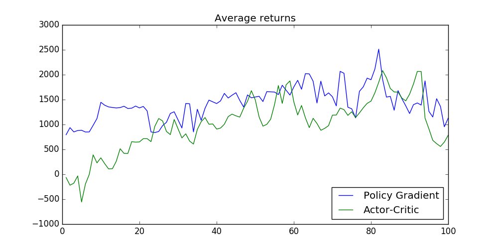
Comparison of average returns from Policy Gradient and Actor-Critic algorithms

As expected, Policy Gradient’s and Actor-Critic’s average returns were close, and Policy Gradient performed slightly better. In addition, Actor-Critic algorithm starts from negative returns initially but significantly improves within the first 10 or 15 iterations.

Comparison of average returns for Actor-Critic and Policy Gradient algorithms

Algorithm Implementation

Please see the GitHub repo for details of the software implementation-

Policy Gradient

Actor-Critic

Computer Vision pipeline

Experiment details

Sawyer’s task is to insert an object into a hole of a specified shape on the surface of a shape sorting cube. Sawyer’s joints right_j3, right_j4, right_j5 were controlled by the policy while other joints were not controlled and maintained in fixed configurations purely for space constraint reasons and for the purpose of avoiding collisions with the environment during training phase.

Goal Specifications

Two goal poses were specified in Sawyer’s workspace. Cartesian coordinates of 3 points on the specified hole of the shape sorting cube are used to identify the pose of the goal. Similarly, Cartesian coordinates of 3 points on the outward facing surface of the object are used to identify the pose of the object. During training, specified goals are iterated through in a round robin fashion with a small amount of gaussian noise added to the goal location.

Initial conditions

At the beginning of each trajectory, along with the selection of a new goal, the joints return to a region contained by a gaussian around the fixed and pre-defined initial joint angles

Reward function

Multiple versions of reward functions were tried in the early stages of development and the following function was finally settled upon as it had the best performance

Reward = w_l2 * l2**2 + w_log * log(l2**2 + α) + w_u * ||u||**2

where l2 is the Eucledian distance between the center of the cyclinder’s circular face towards the shape sorting cube and a point at a fixed height above the center of the circular hole in the shape sorting cube. w_l2 was chosen as 1e-3.

The reward function has the log of the l2 squared distance term to produce higher rewards as the distance between the points becomes closer. alpha was specified as 1e-6, and w_log was chosen as 1.0.

u is the control output vector and w_u was chosen as 1e-2.

Hyperparameter search

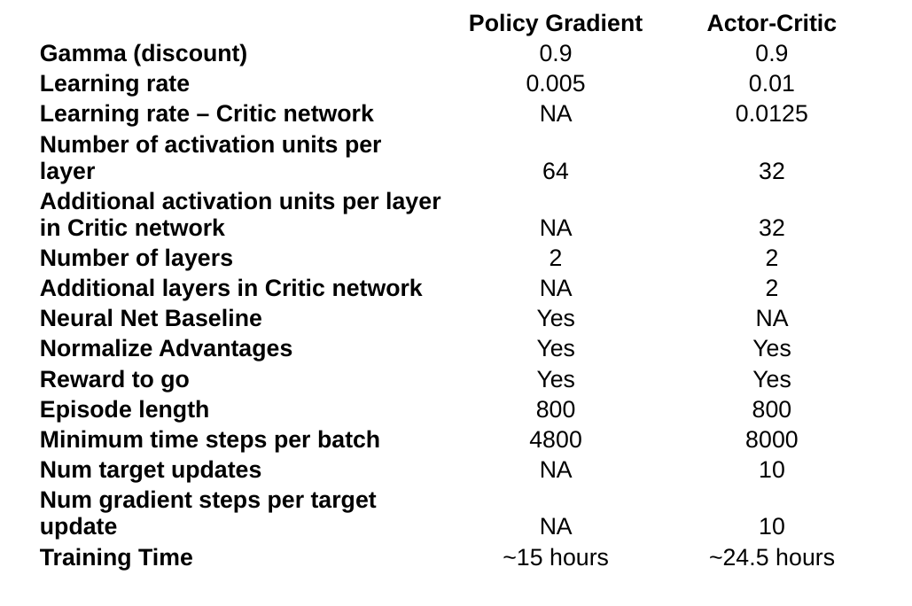
Hyperparameters for Actor-Critic and Policy Gradient algorithms

Both reward to go and advantage normalization options were enabled for both algorithms. Increasing the trajectory length or minimum timesteps per batch only increases the training time and did not necessarily produce a better policy.

For Policy Gradient a reward discount factor of 0.9 and a learning rate of 0.005 worked well. For Actor-Critic a reward discount factor of 0.9 and a learning rate of 0.01 for the actor network and 0.0125 for the critic network worked well.

The policy network consists of tanh activation units for the input and hidden layers and linear activations for the output layer.

Observations (Input to policy)

For velocity control mode

[angle_0, angle_1, …., angle_N, x_object, y_object, z_object, x_goal, y_goal, z_goal]

For torque control mode

[angle_0, angle_1, …., angle_N, vel_0, vel_1, …, vel_N, x_object, y_object, z_object, x_goal, y_goal, z_goal]

where N is the number of joints being controlled

Actions (Output of policy)

For velcoity control mode

[vel_0, vel_1, …., vel_N]